Danger
Please access this document in its canonical location as the currently accessed page may not be rendered correctly: Integrating data using ingest and BBKNN
Integrating data using ingest and BBKNN#
The following tutorial describes a simple PCA-based method for integrating data we call ingest() and compares it with BBKNN [Polanski2019].
BBKNN integrates well with the Scanpy workflow and is accessible through the bbknn() function.
The ingest() function assumes an annotated reference dataset that captures the biological variability of interest.
The rational is to fit a model on the reference data and use it to project new data.
For the time being, this model is a PCA combined with a neighbor lookup search tree, for which we use UMAP’s implementation [McInnes2018].
Similar PCA-based integrations have been used before, for instance, in [Weinreb2020].
As
ingest()is simple and the procedure clear, the workflow is transparent and fast.Like BBKNN,
ingest()leaves the data matrix itself invariant.Unlike BBKNN,
ingest()solves the label mapping problem (like scmap) and maintains an embedding that might have desired properties like specific clusters or trajectories.
We refer to this asymmetric dataset integration as ingesting annotations from an annotated reference adata_ref into an adata that still lacks this annotation.
It is different from learning a joint representation that integrates datasets in a symmetric way as BBKNN, Scanorma, Conos, CCA (e.g. in Seurat) or a conditional VAE (e.g. in scVI, trVAE) would do, but comparable to the initiall MNN implementation in scran.
Take a look at tools in the external API or at the scverse ecosystem to get a start with other tools.
from __future__ import annotations

import anndata
import pandas as pd
import scanpy as sc
sc.settings.verbosity = 1  # verbosity: errors (0), warnings (1), info (2), hints (3)
sc.logging.print_versions()
sc.settings.set_figure_params(dpi=80, frameon=False, figsize=(3, 3), facecolor="white")
-----
anndata     0.10.9
scanpy      1.10.3
-----
Cython              3.0.11
PIL                 10.4.0
asttokens           NA
charset_normalizer  3.3.2
comm                0.2.2
cycler              0.12.1
cython              3.0.11
cython_runtime      NA
dateutil            2.9.0.post0
debugpy             1.8.5
decorator           5.1.1
executing           2.1.0
h5py                3.11.0
igraph              0.11.6
ipykernel           6.29.5
jaraco              NA
jedi                0.19.1
joblib              1.4.2
kiwisolver          1.4.7
legacy_api_wrap     NA
leidenalg           0.10.2
llvmlite            0.43.0
louvain             0.8.2
matplotlib          3.9.2
more_itertools      10.5.0
mpl_toolkits        NA
natsort             8.4.0
numba               0.60.0
numpy               2.0.2
packaging           24.1
pandas              2.2.3
parso               0.8.4
pkg_resources       NA
platformdirs        4.3.3
prompt_toolkit      3.0.47
psutil              6.0.0
pure_eval           0.2.3
pydev_ipython       NA
pydevconsole        NA
pydevd              2.9.5
pydevd_file_utils   NA
pydevd_plugins      NA
pydevd_tracing      NA
pygments            2.18.0
pyparsing           3.1.4
pytz                2024.2
scipy               1.14.1
session_info        1.0.0
six                 1.16.0
sklearn             1.5.2
stack_data          0.6.3
texttable           1.7.0
threadpoolctl       3.5.0
tornado             6.4.1
traitlets           5.14.3
vscode              NA
wcwidth             0.2.13
zmq                 26.2.0
-----
IPython             8.27.0
jupyter_client      8.6.2
jupyter_core        5.7.2
-----
Python 3.12.7 (main, Oct  1 2024, 11:15:50) [GCC 14.2.1 20240910]
Linux-6.11.3-zen1-1-zen-x86_64-with-glibc2.40
-----
Session information updated at 2024-10-14 15:28
PBMCs#
We consider an annotated reference dataset adata_ref and a dataset for which you want to query labels and embeddings adata.
# this is an earlier version of the dataset from the pbmc3k tutorial
adata_ref = sc.datasets.pbmc3k_processed()
adata = sc.datasets.pbmc68k_reduced()
To use sc.tl.ingest, the datasets need to be defined on the same variables.
var_names = adata_ref.var_names.intersection(adata.var_names)
adata_ref = adata_ref[:, var_names].copy()
adata = adata[:, var_names].copy()
The model and graph (here PCA, neighbors, UMAP) trained on the reference data will explain the biological variation observed within it.
sc.pp.pca(adata_ref)
sc.pp.neighbors(adata_ref)
sc.tl.umap(adata_ref)
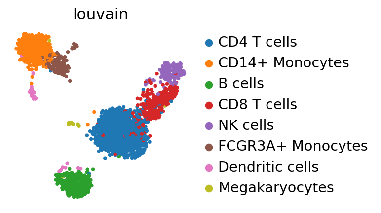
The manifold still looks essentially the same as in the /tutorials/basics/clustering-2017.
sc.pl.umap(adata_ref, color="louvain")
Mapping PBMCs using ingest#
Let’s map labels and embeddings from adata_ref to adata based on a chosen representation. Here, we use adata_ref.obsm['X_pca'] to map cluster labels and the UMAP coordinates.
sc.tl.ingest(adata, adata_ref, obs="louvain")
adata.uns["louvain_colors"] = adata_ref.uns["louvain_colors"] # fix colors
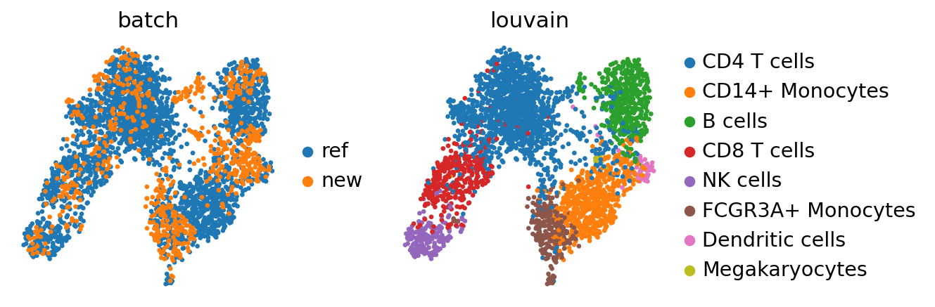
sc.pl.umap(adata, color=["louvain", "bulk_labels"], wspace=0.5)
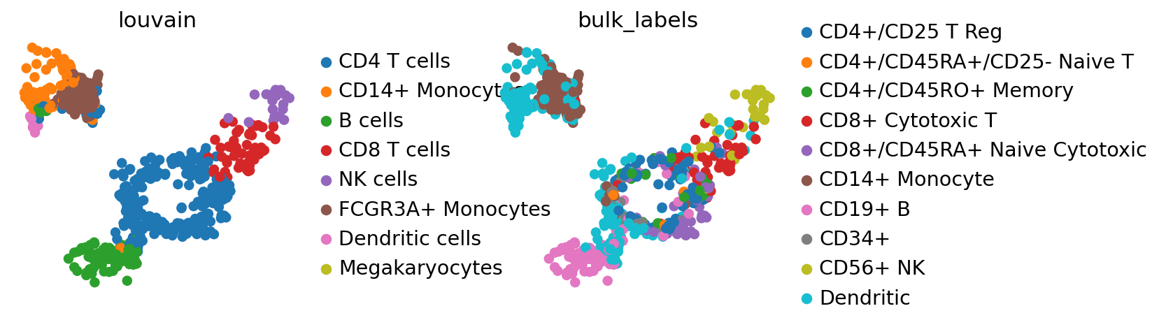
By comparing the ‘bulk_labels’ annotation with ‘louvain’, we see that the data has been reasonably mapped, only the annotation of dendritic cells seems ambiguous and might have been ambiiguous in adata already.
adata_concat = anndata.concat([adata_ref, adata], label="batch", keys=["ref", "new"])
adata_concat.obs["louvain"] = (
    adata_concat.obs["louvain"].astype("category").cat.reorder_categories(adata_ref.obs["louvain"].cat.categories)
)
# fix category colors
adata_concat.uns["louvain_colors"] = adata_ref.uns["louvain_colors"]
sc.pl.umap(adata_concat, color=["batch", "louvain"])
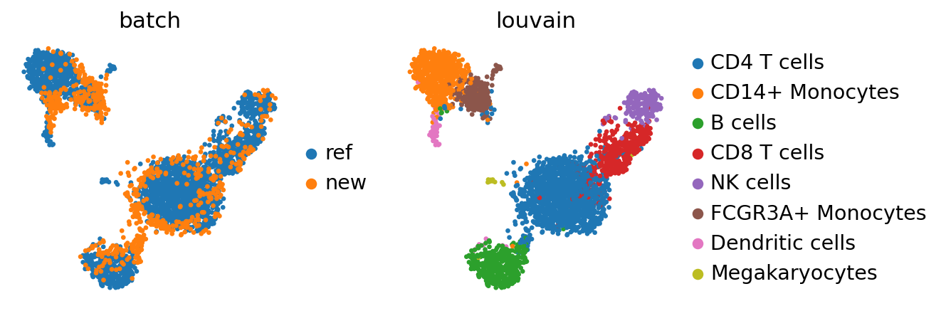
While there seems to be some batch-effect in the monocytes and dendritic cell clusters, the new data is otherwise mapped relatively homogeneously.
The megakaryoctes are only present in adata_ref and no cells from adata map onto them. If interchanging reference data and query data, Megakaryocytes do not appear as a separate cluster anymore. This is an extreme case as the reference data is very small; but one should always question if the reference data contain enough biological variation to meaningfully accomodate query data.
Using BBKNN#
sc.tl.pca(adata_concat)
%%time
sc.external.pp.bbknn(adata_concat, batch_key="batch")  # running bbknn 1.3.6
WARNING: consider updating your call to make use of `computation`
CPU times: user 1.56 s, sys: 19 ms, total: 1.58 s
Wall time: 771 ms
sc.tl.umap(adata_concat)
sc.pl.umap(adata_concat, color=["batch", "louvain"])
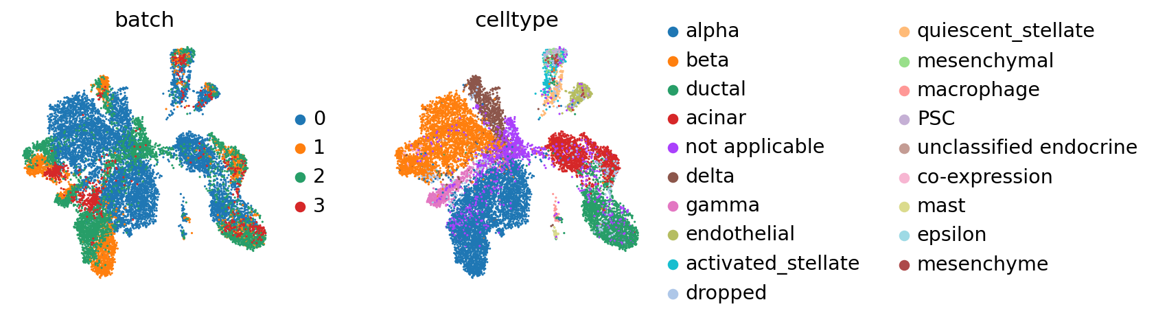
Also BBKNN doesn’t maintain the Megakaryocytes cluster. However, it seems to mix cells more homogeneously.
Pancreas#
The following data has been used in the scGen paper [Lotfollahi2019], has been used here, was curated here and can be downloaded from here (the BBKNN paper).
It contains data for human pancreas from 4 different studies [Segerstolpe2016,Baron2016,Wang2016,Muraro2016], which have been used in the seminal papers on single-cell dataset integration [Butler2018,Haghverdi2018] and many times ever since.
# note that this collection of batches is already intersected on the genes
adata_all = sc.read(
    "data/pancreas.h5ad",
    backup_url="https://www.dropbox.com/s/qj1jlm9w10wmt0u/pancreas.h5ad?dl=1",
)
adata_all.shape
(14693, 2448)
Inspect the cell types observed in these studies.
counts = adata_all.obs["celltype"].value_counts()
counts.to_frame()
| count | |
|---|---|
| celltype | |
| alpha | 4214 |
| beta | 3354 |
| ductal | 1804 |
| acinar | 1368 |
| not applicable | 1154 |
| delta | 917 |
| gamma | 571 |
| endothelial | 289 |
| activated_stellate | 284 |
| dropped | 178 |
| quiescent_stellate | 173 |
| mesenchymal | 80 |
| macrophage | 55 |
| PSC | 54 |
| unclassified endocrine | 41 |
| co-expression | 39 |
| mast | 32 |
| epsilon | 28 |
| mesenchyme | 27 |
| schwann | 13 |
| t_cell | 7 |
| MHC class II | 5 |
| unclear | 4 |
| unclassified | 2 |
To simplify visualization, let’s remove the 5 minority classes.
minority_classes = counts.index[-5:].tolist()  # get the minority classes
# actually subset
adata_all = adata_all[~adata_all.obs["celltype"].isin(minority_classes)].copy()
# reorder according to abundance
adata_all.obs["celltype"] = adata_all.obs["celltype"].cat.reorder_categories(counts.index[:-5].tolist())
Seeing the batch effect#
sc.pp.pca(adata_all)
sc.pp.neighbors(adata_all)
sc.tl.umap(adata_all)
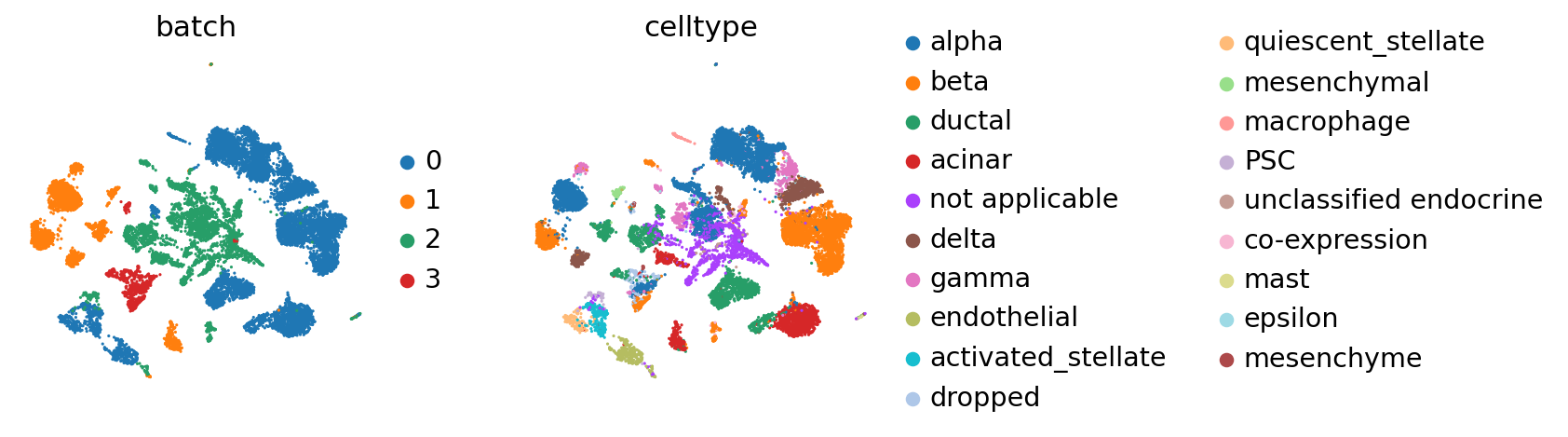
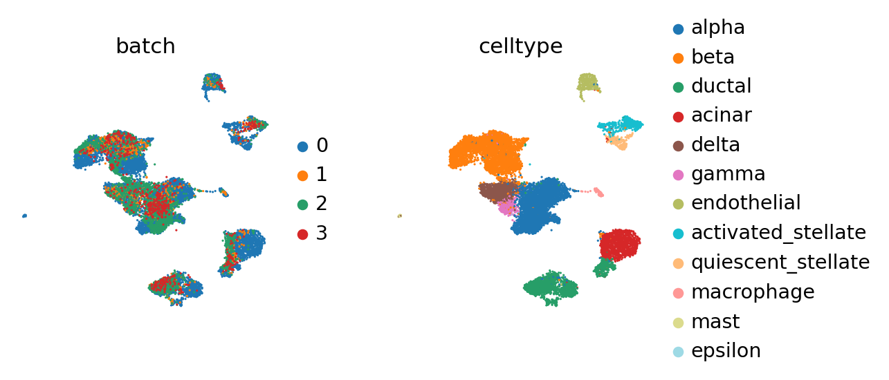
We observe a batch effect.
sc.pl.umap(adata_all, color=["batch", "celltype"], palette=sc.pl.palettes.vega_20_scanpy)
BBKNN#
It can be well-resolved using BBKNN [Polanski2019].
%%time
sc.external.pp.bbknn(adata_all, batch_key="batch")
WARNING: consider updating your call to make use of `computation`
CPU times: user 1.17 s, sys: 24 ms, total: 1.2 s
Wall time: 1.14 s
sc.tl.umap(adata_all)
sc.pl.umap(adata_all, color=["batch", "celltype"])
If one prefers to work more iteratively starting from one reference dataset, one can use ingest.
Mapping onto a reference batch using ingest#
Choose one reference batch for training the model and setting up the neighborhood graph (here, a PCA) and separate out all other batches.
As before, the model trained on the reference batch will explain the biological variation observed within it.
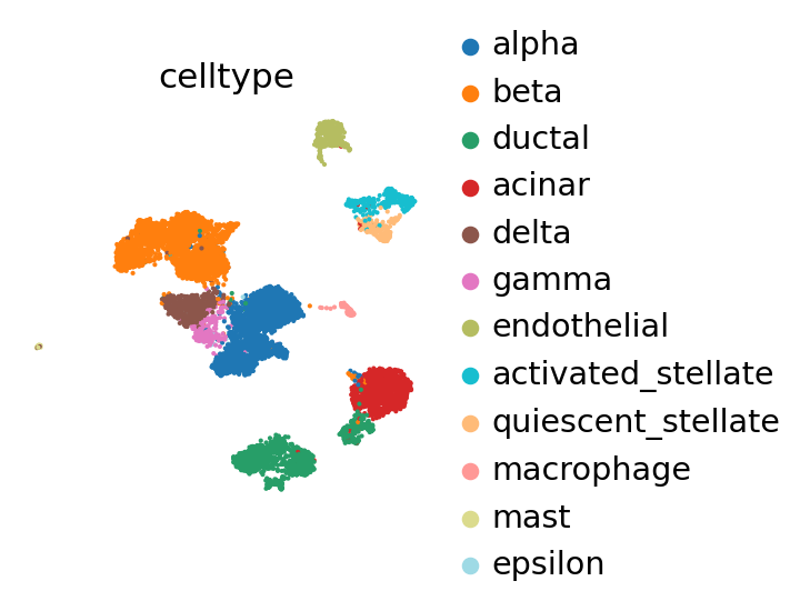
adata_ref = adata_all[adata_all.obs["batch"] == "0"].copy()
Compute the PCA, neighbors and UMAP on the reference data.
sc.pp.pca(adata_ref)
sc.pp.neighbors(adata_ref)
sc.tl.umap(adata_ref)
The reference batch contains 12 of the 19 cell types across all batches.
sc.pl.umap(adata_ref, color="celltype")
Iteratively map labels (such as ‘celltype’) and embeddings (such as ‘X_pca’ and ‘X_umap’) from the reference data onto the query batches.
adatas = [adata_all[adata_all.obs["batch"] == i].copy() for i in ["1", "2", "3"]]
sc.settings.verbosity = 2  # a bit more logging
for iadata, adata in enumerate(adatas, 1):
    print(f"... integrating batch {iadata}")
    adata.obs["celltype_orig"] = adata.obs["celltype"]  # save the original cell type
    sc.tl.ingest(adata, adata_ref, obs="celltype")
... integrating batch 1
running ingest
    finished (0:00:02)
... integrating batch 2
running ingest
    finished (0:00:03)
... integrating batch 3
running ingest
finished (0:00:01)
Each of the query batches now carries annotation that has been contextualized with adata_ref. By concatenating, we can view it together.
adata_concat = anndata.concat([adata_ref, *adatas], label="batch", join="outer")
adata_concat.obs["celltype"] = (
    adata_concat.obs["celltype"].astype("category").cat.reorder_categories(adata_ref.obs["celltype"].cat.categories)
)
# fix category coloring
adata_concat.uns["celltype_colors"] = adata_ref.uns["celltype_colors"]
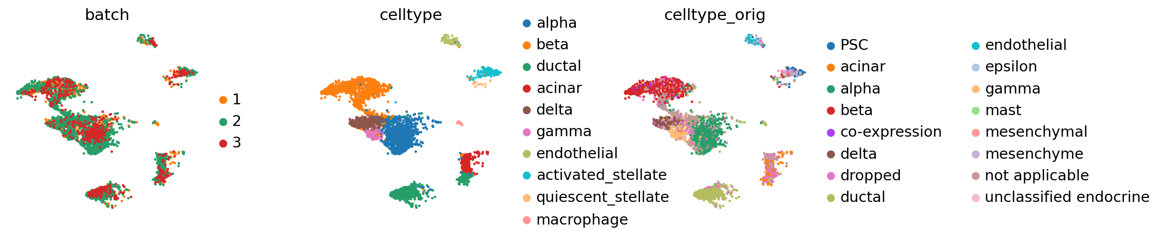
sc.pl.umap(adata_concat, color=["batch", "celltype"])
Compared to the BBKNN result, this is maintained clusters in a much more pronounced fashion. If one already observed a desired continuous structure (as in the hematopoietic datasets, for instance), ingest allows to easily maintain this structure.
Evaluating consistency#
Let us subset the data to the query batches.
adata_query = adata_concat[adata_concat.obs["batch"].isin(["1", "2", "3"])].copy()
The following plot is a bit hard to read, hence, move on to confusion matrices below.
sc.pl.umap(adata_query, color=["batch", "celltype", "celltype_orig"], wspace=0.4)
Cell types conserved across batches#
Let us first focus on cell types that are conserved with the reference, to simplify reading of the confusion matrix.
# intersected categories
conserved_categories = adata_query.obs["celltype"].cat.categories.intersection(
    adata_query.obs["celltype_orig"].cat.categories
)
# intersect categories
obs_query_conserved = adata_query.obs.loc[
    adata_query.obs["celltype"].isin(conserved_categories) & adata_query.obs["celltype_orig"].isin(conserved_categories)
].copy()
# remove unused categories
obs_query_conserved["celltype"] = obs_query_conserved["celltype"].cat.remove_unused_categories()
# remove unused categories and fix category ordering
obs_query_conserved["celltype_orig"] = (
    obs_query_conserved["celltype_orig"]
    .cat.remove_unused_categories()
    .cat.reorder_categories(obs_query_conserved["celltype"].cat.categories)
)
pd.crosstab(obs_query_conserved["celltype"], obs_query_conserved["celltype_orig"])
| celltype_orig | alpha | beta | ductal | acinar | delta | gamma | endothelial |
|---|---|---|---|---|---|---|---|
| celltype | |||||||
| alpha | 1814 | 3 | 16 | 1 | 1 | 20 | 0 |
| beta | 53 | 805 | 6 | 1 | 11 | 35 | 0 |
| ductal | 7 | 5 | 681 | 241 | 0 | 0 | 0 |
| acinar | 2 | 3 | 3 | 165 | 0 | 3 | 0 |
| delta | 6 | 3 | 2 | 0 | 304 | 71 | 0 |
| gamma | 1 | 5 | 0 | 1 | 0 | 187 | 0 |
| endothelial | 2 | 0 | 0 | 0 | 0 | 0 | 36 |
Overall, the conserved cell types are also mapped as expected. The main exception are some acinar cells in the original annotation that appear as acinar cells. However, already the reference data is observed to feature a cluster of both acinar and ductal cells, which explains the discrepancy, and indicates a potential inconsistency in the initial annotation.
All cell types#
Let us now move on to look at all cell types.
pd.crosstab(adata_query.obs["celltype"], adata_query.obs["celltype_orig"])
| celltype_orig | PSC | acinar | alpha | beta | co-expression | delta | dropped | ductal | endothelial | epsilon | gamma | mast | mesenchymal | mesenchyme | not applicable | unclassified endocrine |
|---|---|---|---|---|---|---|---|---|---|---|---|---|---|---|---|---|
| celltype | ||||||||||||||||
| alpha | 0 | 1 | 1814 | 3 | 2 | 1 | 40 | 16 | 0 | 3 | 20 | 7 | 0 | 0 | 312 | 10 |
| beta | 1 | 1 | 53 | 805 | 37 | 11 | 41 | 6 | 0 | 0 | 35 | 0 | 0 | 1 | 522 | 24 |
| ductal | 0 | 241 | 7 | 5 | 0 | 0 | 37 | 681 | 0 | 0 | 0 | 0 | 2 | 0 | 94 | 0 |
| acinar | 0 | 165 | 2 | 3 | 0 | 0 | 23 | 3 | 0 | 0 | 3 | 0 | 0 | 0 | 90 | 0 |
| delta | 0 | 0 | 6 | 3 | 0 | 304 | 13 | 2 | 0 | 6 | 71 | 0 | 0 | 0 | 95 | 7 |
| gamma | 0 | 1 | 1 | 5 | 0 | 0 | 2 | 0 | 0 | 1 | 187 | 0 | 0 | 0 | 15 | 0 |
| endothelial | 1 | 0 | 2 | 0 | 0 | 0 | 6 | 0 | 36 | 0 | 0 | 0 | 0 | 6 | 7 | 0 |
| activated_stellate | 48 | 1 | 1 | 3 | 0 | 0 | 11 | 6 | 0 | 0 | 0 | 0 | 78 | 20 | 17 | 0 |
| quiescent_stellate | 4 | 0 | 1 | 1 | 0 | 0 | 5 | 1 | 1 | 0 | 0 | 0 | 0 | 0 | 1 | 0 |
| macrophage | 0 | 0 | 1 | 1 | 0 | 0 | 0 | 12 | 0 | 0 | 0 | 0 | 0 | 0 | 1 | 0 |
We observe that PSC (pancreatic stellate cells) cells are in fact just inconsistently annotated and correctly mapped on ‘activated_stellate’ cells.
Also, it’s nice to see that ‘mesenchyme’ and ‘mesenchymal’ cells both map onto the same category. However, that category is again ‘activated_stellate’ and likely incorrect.
Visualizing distributions across batches#
Often, batches correspond to experiments that one wants to compare. Scanpy offers to convenient visualization possibilities for this.
a density plot
a partial visualization of a subset of categories/groups in an emnbedding
Density plot#
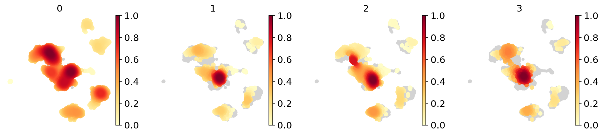
sc.tl.embedding_density(adata_concat, groupby="batch")
computing density on 'umap'
sc.pl.embedding_density(adata_concat, groupby="batch")
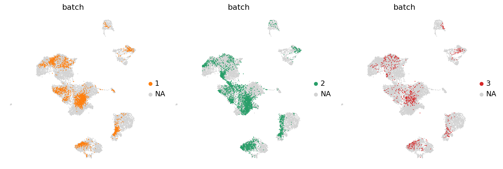
Partial visualizaton of a subset of groups in embedding#
import matplotlib.pyplot as plt


fig, axes = plt.subplots(1, 3, figsize=(15, 5))
for batch, ax in zip(["1", "2", "3"], axes, strict=True):
    sc.pl.umap(adata_concat, color="batch", groups=[batch], ax=ax, show=False)