Integrating spatial data with scRNA-seq using scanorama#
Author: Giovanni Palla
Note
For up-to-date analysis tutorials, kindly check out SquidPy tutorials.
This tutorial shows how to work with multiple Visium datasets and perform integration of scRNA-seq dataset with Scanpy. It follows the previous tutorial on analysis and visualization of spatial transcriptomics data.
We will use Scanorama paper - code to perform integration and label transfer. It has a convenient interface with scanpy and anndata.
To install the required libraries, type the following:
pip install git+https://github.com/theislab/scanpy.git
pip install git+https://github.com/theislab/anndata.git
pip install scanorama
Loading libraries#
from __future__ import annotations

from pathlib import Path

import anndata as an
import matplotlib.pyplot as plt
import numpy as np
import pandas as pd
import scanorama
import scanpy as sc
import seaborn as sns
sc.logging.print_versions()
sc.set_figure_params(facecolor="white", figsize=(8, 8))
sc.settings.verbosity = 3
-----
anndata     0.11.0.dev78+g64ab900
scanpy      1.10.0rc2.dev6+g14555ba4
-----
PIL                         10.2.0
annoy                       NA
anyio                       NA
appnope                     0.1.3
arrow                       1.3.0
asciitree                   NA
asttokens                   NA
attr                        23.2.0
attrs                       23.2.0
babel                       2.14.0
certifi                     2023.11.17
cffi                        1.16.0
charset_normalizer          3.3.2
cloudpickle                 3.0.0
comm                        0.2.1
cycler                      0.12.1
cython_runtime              NA
dask                        2024.1.0
dateutil                    2.8.2
debugpy                     1.8.0
decorator                   5.1.1
defusedxml                  0.7.1
executing                   2.0.1
fasteners                   0.19
fastjsonschema              NA
fbpca                       NA
fqdn                        NA
h5py                        3.10.0
idna                        3.6
igraph                      0.10.8
intervaltree                NA
ipykernel                   6.28.0
ipywidgets                  8.1.1
isoduration                 NA
jedi                        0.19.1
jinja2                      3.1.3
joblib                      1.3.2
json5                       NA
jsonpointer                 2.4
jsonschema                  4.20.0
jsonschema_specifications   NA
jupyter_events              0.9.0
jupyter_server              2.12.4
jupyterlab_server           2.25.2
kiwisolver                  1.4.5
legacy_api_wrap             NA
leidenalg                   0.10.1
llvmlite                    0.41.1
markupsafe                  2.1.3
matplotlib                  3.8.2
mpl_toolkits                NA
msgpack                     1.0.7
natsort                     8.4.0
nbformat                    5.9.2
numba                       0.58.1
numcodecs                   0.12.1
numpy                       1.26.3
overrides                   NA
packaging                   23.2
pandas                      2.2.0
parso                       0.8.3
patsy                       0.5.6
pexpect                     4.9.0
platformdirs                4.1.0
prometheus_client           NA
prompt_toolkit              3.0.43
psutil                      5.9.7
ptyprocess                  0.7.0
pure_eval                   0.2.2
pydev_ipython               NA
pydevconsole                NA
pydevd                      2.9.5
pydevd_file_utils           NA
pydevd_plugins              NA
pydevd_tracing              NA
pygments                    2.17.2
pyparsing                   3.1.1
pythonjsonlogger            NA
pytz                        2023.3.post1
referencing                 NA
requests                    2.31.0
rfc3339_validator           0.1.4
rfc3986_validator           0.1.1
rpds                        NA
scanorama                   1.7.4
scipy                       1.11.4
seaborn                     0.13.1
send2trash                  NA
session_info                1.0.0
setuptools                  68.2.2
setuptools_scm              NA
sitecustomize               NA
six                         1.16.0
sklearn                     1.3.2
sniffio                     1.3.0
sortedcontainers            2.4.0
sparse                      0.15.1
stack_data                  0.6.3
statsmodels                 0.14.1
tblib                       3.0.0
texttable                   1.7.0
threadpoolctl               3.2.0
tlz                         0.12.0
toolz                       0.12.0
tornado                     6.4
traitlets                   5.14.1
typing_extensions           NA
uri_template                NA
urllib3                     2.1.0
wcwidth                     0.2.13
webcolors                   1.13
websocket                   1.7.0
yaml                        6.0.1
zarr                        2.16.1
zipp                        NA
zmq                         25.1.2
-----
IPython             8.20.0
jupyter_client      8.6.0
jupyter_core        5.7.1
jupyterlab          4.0.10
notebook            7.0.6
-----
Python 3.11.6 (main, Nov  2 2023, 04:39:43) [Clang 14.0.3 (clang-1403.0.22.14.1)]
macOS-13.6.1-arm64-arm-64bit
-----
Session information updated at 2024-02-26 13:25
Reading the data#
We will use two Visium spatial transcriptomics dataset of the mouse brain (Sagittal), which are publicly available from the 10x genomics website.
The function datasets.visium_sge() downloads the dataset from 10x genomics and returns an AnnData object that contains counts, images and spatial coordinates. We will calculate standards QC metrics with pp.calculate_qc_metrics and visualize them.
When using your own Visium data, use squidpy.read.visium() to import it.
adata_spatial_anterior = sc.datasets.visium_sge(sample_id="V1_Mouse_Brain_Sagittal_Anterior")
adata_spatial_posterior = sc.datasets.visium_sge(sample_id="V1_Mouse_Brain_Sagittal_Posterior")
reading /Users/ilangold/Projects/Theis/scanpy-tutorials/spatial/data/V1_Mouse_Brain_Sagittal_Anterior/filtered_feature_bc_matrix.h5
 (0:00:01)
reading /Users/ilangold/Projects/Theis/scanpy-tutorials/spatial/data/V1_Mouse_Brain_Sagittal_Posterior/filtered_feature_bc_matrix.h5
 (0:00:01)
adata_spatial_anterior.var_names_make_unique()
adata_spatial_posterior.var_names_make_unique()
sc.pp.calculate_qc_metrics(adata_spatial_anterior, inplace=True)
sc.pp.calculate_qc_metrics(adata_spatial_posterior, inplace=True)
for name, adata in [
    ("anterior", adata_spatial_anterior),
    ("posterior", adata_spatial_posterior),
]:
    fig, axs = plt.subplots(1, 4, figsize=(12, 3))
    fig.suptitle(f"Covariates for filtering: {name}")

    sns.histplot(adata.obs["total_counts"], kde=False, ax=axs[0])
    sns.histplot(
        adata.obs["total_counts"][adata.obs["total_counts"] < 20000],
        kde=False,
        bins=40,
        ax=axs[1],
    )
    sns.histplot(adata.obs["n_genes_by_counts"], kde=False, bins=60, ax=axs[2])
    sns.histplot(
        adata.obs["n_genes_by_counts"][adata.obs["n_genes_by_counts"] < 4000],
        kde=False,
        bins=60,
        ax=axs[3],
    )
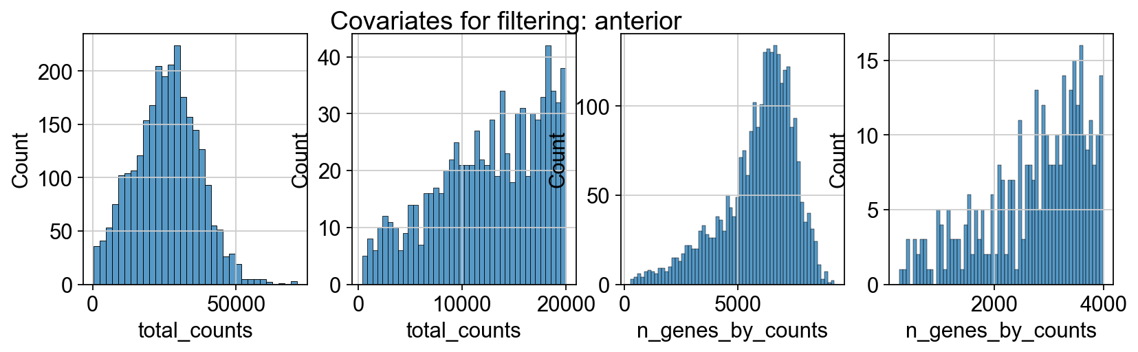
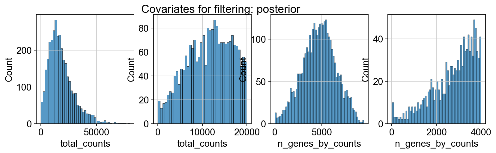
sc.datasets.visium_sge downloads the filtered visium dataset, the output of spaceranger that contains only spots within the tissue slice. Indeed, looking at standard QC metrics we can observe that the samples do not contain empty spots.
We proceed to normalize Visium counts data with the built-in normalize_total method from Scanpy, and detect highly-variable genes (for later). As discussed previously, note that there are more sensible alternatives for normalization (see discussion in sc-tutorial paper and more recent alternatives such as SCTransform or GLM-PCA).
for adata in [
    adata_spatial_anterior,
    adata_spatial_posterior,
]:
    sc.pp.normalize_total(adata, inplace=True)
    sc.pp.log1p(adata)
    sc.pp.highly_variable_genes(adata, flavor="seurat", n_top_genes=2000, inplace=True)
normalizing counts per cell
    finished (0:00:00)
extracting highly variable genes
    finished (0:00:00)
--> added
    'highly_variable', boolean vector (adata.var)
    'means', float vector (adata.var)
    'dispersions', float vector (adata.var)
    'dispersions_norm', float vector (adata.var)
normalizing counts per cell
    finished (0:00:00)
extracting highly variable genes
    finished (0:00:00)
--> added
    'highly_variable', boolean vector (adata.var)
    'means', float vector (adata.var)
    'dispersions', float vector (adata.var)
    'dispersions_norm', float vector (adata.var)
Data integration#
We are now ready to perform integration of the two dataset. As mentioned before, we will be using Scanorama for that. Scanorama returns two lists, one for the integrated embeddings and one for the corrected counts, for each dataset.
We would like to note that in this context using scanpy.external.pp.bbknn() or scanpy.tl.ingest() is also possible.
adatas = [adata_spatial_anterior, adata_spatial_posterior]
adatas_cor = scanorama.correct_scanpy(adatas, return_dimred=True)
Found 32285 genes among all datasets
[[0.         0.48882265]
 [0.         0.        ]]
Processing datasets (0, 1)
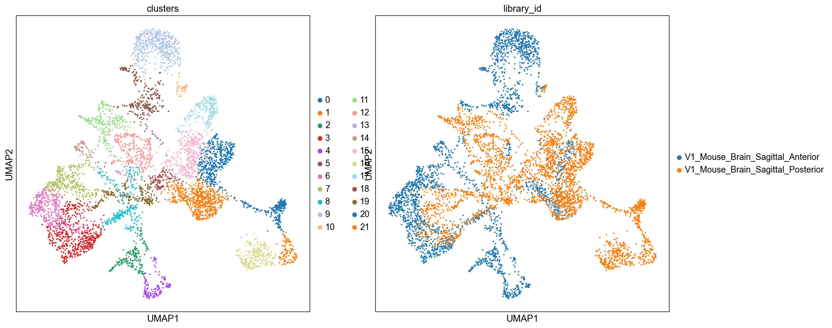
We will concatenate the two datasets and save the integrated embeddings in adata_spatial.obsm['scanorama_embedding']. Furthermore we will compute UMAP to visualize the results and qualitatively assess the data integration task.
Notice that we are concatenating the two dataset with uns_merge="unique" strategy, in order to keep both images from the visium datasets in the concatenated anndata object.
adata_spatial = sc.concat(
    adatas_cor,
    label="library_id",
    uns_merge="unique",
    keys=[
        k
        for d in [
            adatas_cor[0].uns["spatial"],
            adatas_cor[1].uns["spatial"],
        ]
        for k, v in d.items()
    ],
    index_unique="-",
)
sc.pp.neighbors(adata_spatial, use_rep="X_scanorama")
sc.tl.umap(adata_spatial)
sc.tl.leiden(adata_spatial, key_added="clusters", n_iterations=2, flavor="igraph", directed=False)
computing neighbors
    finished: added to `.uns['neighbors']`
    `.obsp['distances']`, distances for each pair of neighbors
    `.obsp['connectivities']`, weighted adjacency matrix (0:00:02)
computing UMAP
    finished: added
    'X_umap', UMAP coordinates (adata.obsm) (0:00:06)
running Leiden clustering
    finished: found 22 clusters and added
    'clusters', the cluster labels (adata.obs, categorical) (0:00:00)
sc.pl.umap(adata_spatial, color=["clusters", "library_id"], palette=sc.pl.palettes.default_20)
WARNING: Length of palette colors is smaller than the number of categories (palette length: 20, categories length: 22. Some categories will have the same color.
We can also visualize the clustering result in spatial coordinates. For that, we first need to save the cluster colors in a dictionary. We can then plot the Visium tissue fo the Anterior and Posterior Sagittal view, alongside each other.
clusters_colors = dict(zip([str(i) for i in range(18)], adata_spatial.uns["clusters_colors"], strict=True))
fig, axs = plt.subplots(1, 2, figsize=(15, 10))

for i, library in enumerate(["V1_Mouse_Brain_Sagittal_Anterior", "V1_Mouse_Brain_Sagittal_Posterior"]):
    ad = adata_spatial[adata_spatial.obs.library_id == library, :].copy()
    sc.pl.spatial(
        ad,
        img_key="hires",
        library_id=library,
        color="clusters",
        size=1.5,
        palette=[v for k, v in clusters_colors.items() if k in ad.obs.clusters.unique().tolist()],
        legend_loc=None,
        show=False,
        ax=axs[i],
    )

plt.tight_layout()
WARNING: Length of palette colors is smaller than the number of categories (palette length: 16, categories length: 18. Some categories will have the same color.
WARNING: Length of palette colors is smaller than the number of categories (palette length: 14, categories length: 18. Some categories will have the same color.
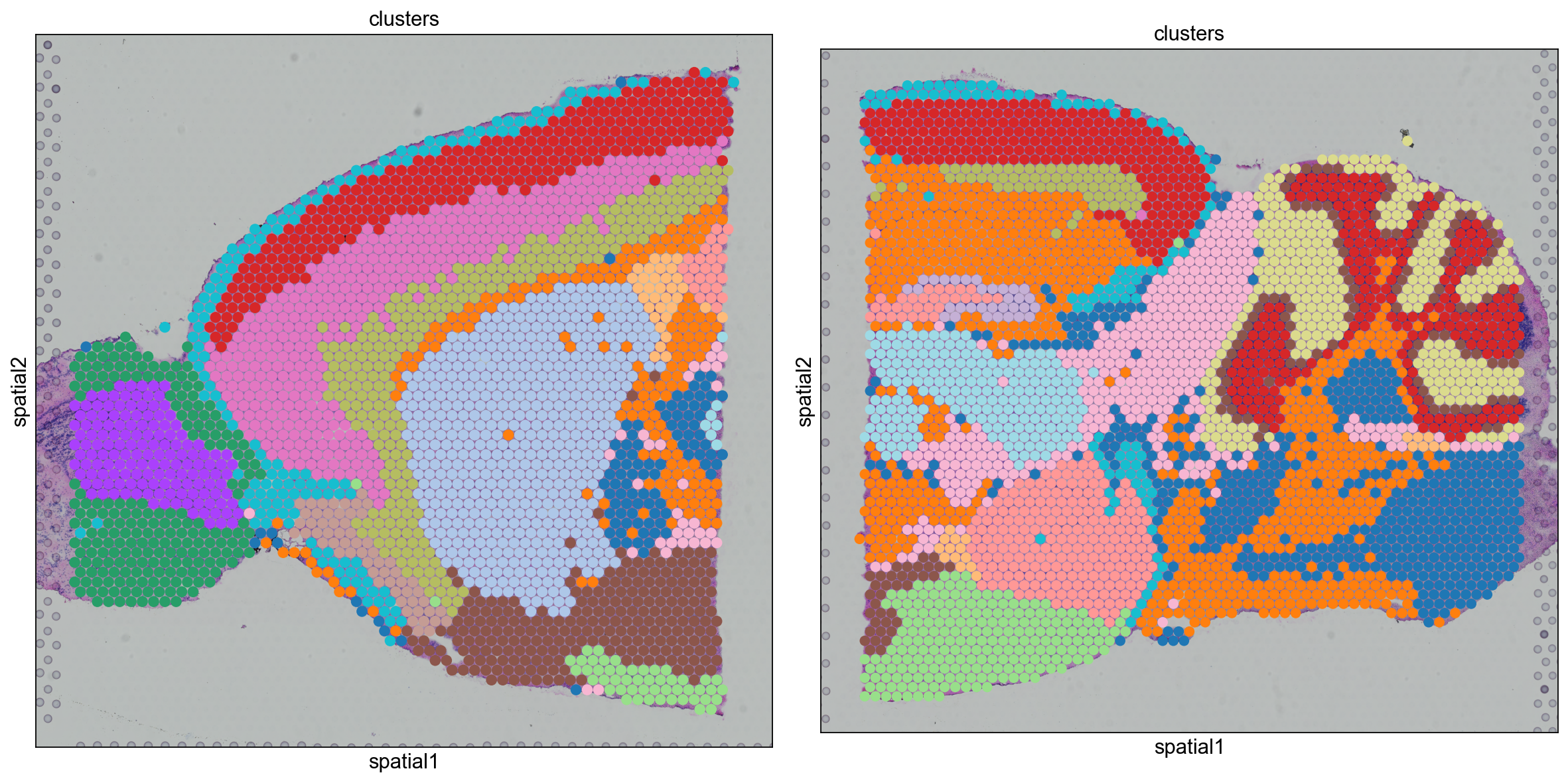
From the clusters, we can clearly see the stratification of the cortical layer in both of the tissues (see the Allen brain atlas for reference). Furthermore, it seems that the dataset integration worked well, since there is a clear continuity between clusters in the two tissues.
Data integration and label transfer from scRNA-seq dataset#
We can also perform data integration between one scRNA-seq dataset and one spatial transcriptomics dataset. Such task is particularly useful because it allows us to transfer cell type labels to the Visium dataset, which were dentified from the scRNA-seq dataset.
For this task, we will be using a dataset from Tasic et al., where the mouse cortex was profiled with smart-seq technology.
The dataset can be downloaded from GEO count - metadata. Conveniently, you can also download the pre-processed dataset in h5ad format from here.
Since the dataset was generated from the mouse cortex, we will subset the visium dataset in order to select only the spots part of the cortex. Note that the integration can also be performed on the whole brain slice, but it would give rise to false positive cell type assignments and and therefore it should be interpreted with more care.
The integration task will be performed with Scanorama: each Visium dataset will be integrated with the smart-seq cortex dataset.
The following cell should be uncommented out and run if this is the first time running this notebook.
if not Path("cache/adata_processed.h5ad").exists():
    import pooch

    p_counts = Path(
        pooch.retrieve(
            "https://ftp.ncbi.nlm.nih.gov/geo/series/GSE115nnn/GSE115746/suppl/GSE115746_cells_exon_counts.csv.gz",
            known_hash="sha256:5693f546dde28680d49bd7bf1255d42b0f77901aec050b94d56e54be10c00648",
            path="../data",
        )
    )
    p_meta = Path(
        pooch.retrieve(
            "https://ftp.ncbi.nlm.nih.gov/geo/series/GSE115nnn/GSE115746/suppl/GSE115746_complete_metadata_28706-cells.csv.gz",
            known_hash="sha256:381cc4dd26898016d506394b4cfbcebab38ac88d2f512ccf98216a5487db5bd2",
            path="../data",
        )
    )

    counts = pd.read_csv(p_counts, compression="gzip", index_col=0).T
    meta = pd.read_csv(p_meta, compression="gzip", index_col="sample_name")
    meta = meta.loc[counts.index]
    annot = sc.queries.biomart_annotations(
        "mmusculus",
        ["mgi_symbol", "ensembl_gene_id"],
    ).set_index("mgi_symbol")
    annot = annot[annot.index.isin(counts.columns)]
    counts = counts.rename(columns=dict(zip(annot.index, annot["ensembl_gene_id"], strict=True)))
    adata_cortex = an.AnnData(counts, obs=meta)
    sc.pp.normalize_total(adata_cortex, inplace=True)
    sc.pp.log1p(adata_cortex)
    adata_cortex.write_h5ad("cache/adata_processed.h5ad")
adata_cortex = sc.read("cache/adata_processed.h5ad")
adata_spatial_anterior.var_names = adata_spatial_anterior.var["gene_ids"]
adata_spatial_posterior.var_names = adata_spatial_posterior.var["gene_ids"]
Subset the spatial anndata to (approximately) selects only spots belonging to the cortex.
adata_anterior_subset = adata_spatial_anterior[adata_spatial_anterior.obsm["spatial"][:, 1] < 6000, :]
adata_posterior_subset = adata_spatial_posterior[
    (adata_spatial_posterior.obsm["spatial"][:, 1] < 4000) & (adata_spatial_posterior.obsm["spatial"][:, 0] < 6000),
    :,
]
Run integration with Scanorama
adatas_anterior = [adata_cortex, adata_anterior_subset]
adatas_posterior = [adata_cortex, adata_posterior_subset]


# Integration.
adatas_cor_anterior = scanorama.correct_scanpy(adatas_anterior, return_dimred=True)
adatas_cor_posterior = scanorama.correct_scanpy(adatas_posterior, return_dimred=True)
Found 22689 genes among all datasets
[[0.         0.22877847]
 [0.         0.        ]]
Processing datasets (0, 1)
Found 22689 genes among all datasets
[[0.         0.35810811]
 [0.         0.        ]]
Processing datasets (0, 1)
Concatenate datasets and assign integrated embeddings to anndata objects.
Notice that we are concatenating datasets with the join="outer" and uns_merge="first" strategies. This is because we want to keep the obsm['coords'] as well as the images of the visium datasets.
adata_cortex_anterior = sc.concat(
    adatas_cor_anterior,
    label="dataset",
    keys=["smart-seq", "visium"],
    join="outer",
    uns_merge="first",
)
adata_cortex_posterior = sc.concat(
    adatas_cor_posterior,
    label="dataset",
    keys=["smart-seq", "visium"],
    join="outer",
    uns_merge="first",
)
At this step, we have integrated each visium dataset in a common embedding with the scRNA-seq dataset. In such embedding space, we can compute distances between samples and use such distances as weights to be used for for propagating labels from the scRNA-seq dataset to the Visium dataset.
Such approach is very similar to the TransferData function in Seurat (see paper). Here, we re-implement the label transfer function with a simple python function, see below.
Frist, let’s compute cosine distances between the visium dataset and the scRNA-seq dataset, in the common embedding space
from sklearn.metrics.pairwise import cosine_distances


distances_anterior = 1 - cosine_distances(
    adata_cortex_anterior[adata_cortex_anterior.obs.dataset == "smart-seq"].obsm["X_scanorama"],
    adata_cortex_anterior[adata_cortex_anterior.obs.dataset == "visium"].obsm["X_scanorama"],
)
distances_posterior = 1 - cosine_distances(
    adata_cortex_posterior[adata_cortex_posterior.obs.dataset == "smart-seq"].obsm["X_scanorama"],
    adata_cortex_posterior[adata_cortex_posterior.obs.dataset == "visium"].obsm["X_scanorama"],
)
Then, let’s propagate labels from the scRNA-seq dataset to the visium dataset
def label_transfer(dist: np.ndarray, labels: pd.Series) -> np.ndarray:
    lab = pd.get_dummies(labels).to_numpy().T
    class_prob = lab @ dist
    norm = np.linalg.norm(class_prob, 2, axis=0)
    class_prob = class_prob / norm
    return (class_prob.T - class_prob.min(1)) / class_prob.ptp(1)
class_prob_anterior = label_transfer(distances_anterior, adata_cortex.obs["cell_subclass"])
class_prob_posterior = label_transfer(distances_posterior, adata_cortex.obs["cell_subclass"])
The class_prob_[anterior-posterior] objects is a numpy array of shape (cell_type, visium_spots) that contains assigned weights of each spots to each cell types. This value essentially tells us how similar that spots look like, from an expression profile perspective, to all the other annotated cell types from the scRNA-seq dataset.
We convert the class_prob_[anterior-posterior] object to a dataframe and assign it to the respective anndata
cp_anterior_df = pd.DataFrame(
    class_prob_anterior,
    columns=sorted(adata_cortex.obs["cell_subclass"].cat.categories),
)
cp_posterior_df = pd.DataFrame(
    class_prob_posterior,
    columns=sorted(adata_cortex.obs["cell_subclass"].cat.categories),
)

cp_anterior_df.index = adata_anterior_subset.obs.index
cp_posterior_df.index = adata_posterior_subset.obs.index
adata_anterior_subset_transfer = adata_anterior_subset.copy()
adata_anterior_subset_transfer.obs = pd.concat([adata_anterior_subset.obs, cp_anterior_df], axis=1)

adata_posterior_subset_transfer = adata_posterior_subset.copy()
adata_posterior_subset_transfer.obs = pd.concat([adata_posterior_subset.obs, cp_posterior_df], axis=1)
We are then able to explore how cell types are propagated from the scRNA-seq dataset to the visium dataset. Let’s first visualize the neurons cortical layers.
sc.pl.spatial(
    adata_anterior_subset_transfer,
    img_key="hires",
    color=["L2/3 IT", "L4", "L5 PT", "L6 CT"],
    size=1.5,
)
sc.pl.spatial(
    adata_posterior_subset_transfer,
    img_key="hires",
    color=["L2/3 IT", "L4", "L5 PT", "L6 CT"],
    size=1.5,
)
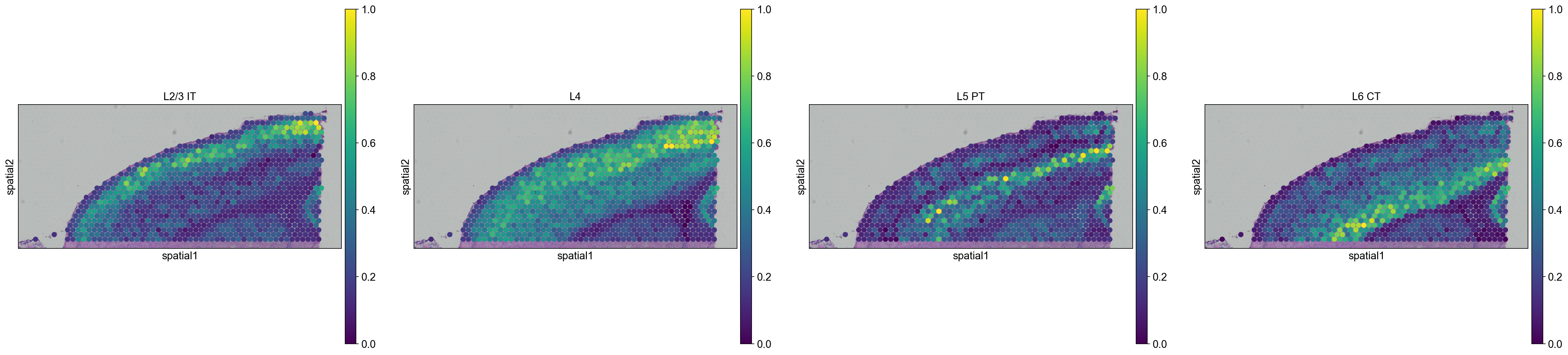
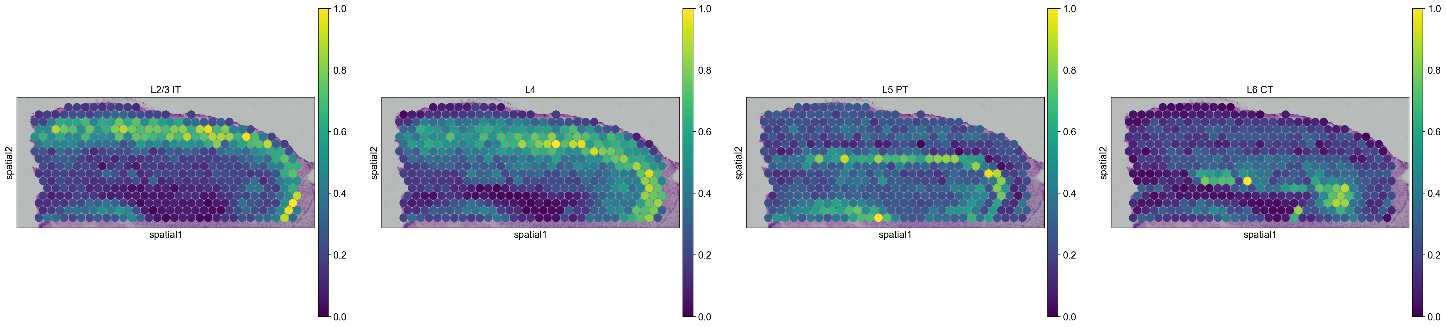
Interestingly, it seems that this approach worked, since sequential layers of cortical neurons could be correctly identified, both in the anterior and posterior sagittal slide.
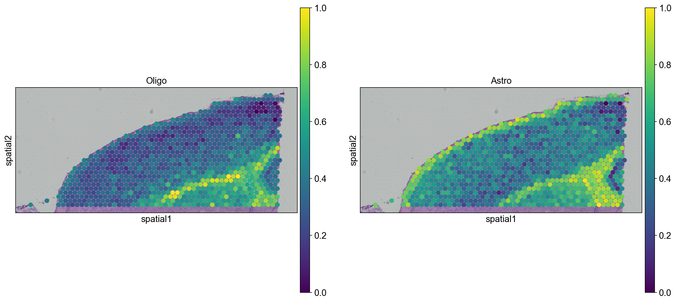
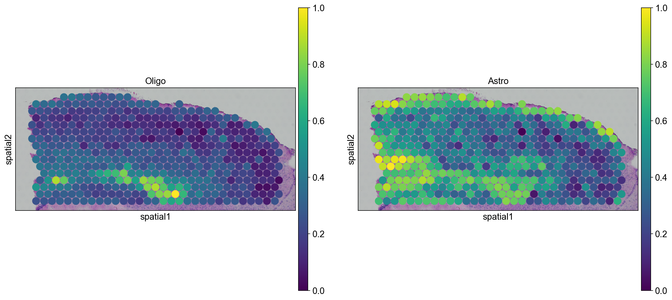
We can go ahead an visualize astrocytes and oligodendrocytes as well.
sc.pl.spatial(adata_anterior_subset_transfer, img_key="hires", color=["Oligo", "Astro"], size=1.5)
sc.pl.spatial(adata_posterior_subset_transfer, img_key="hires", color=["Oligo", "Astro"], size=1.5)
In this tutorial, we showed how to work with multiple slices in Scanpy, and perform label transfers between an annotated scRNA-seq dataset and an unannotated Visium dataset. We showed that such approach, that leverages the data integration performances of Scanorama, is useful and provide a straightforward tool for exploratory analysis.
However, for the label transfer task, we advise analysts to explore more principled approaches, based on cell-type deconvolution, that are likely to provide more accurate and interpretable results. See recent approaches such as: